A Travelling Salesman problem asks which is the shortest possible route that visits each city and returns to the origin city from a given list of cities. It is an NP-Hard problem, which means it is computationally difficult. It is a problem easy to state, difficult to solve. TSP finds its application in vehicle routing, PCB/IC Design etc.

Christofides Algorithm:

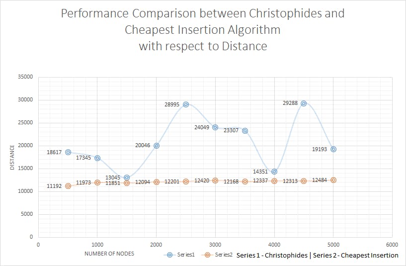
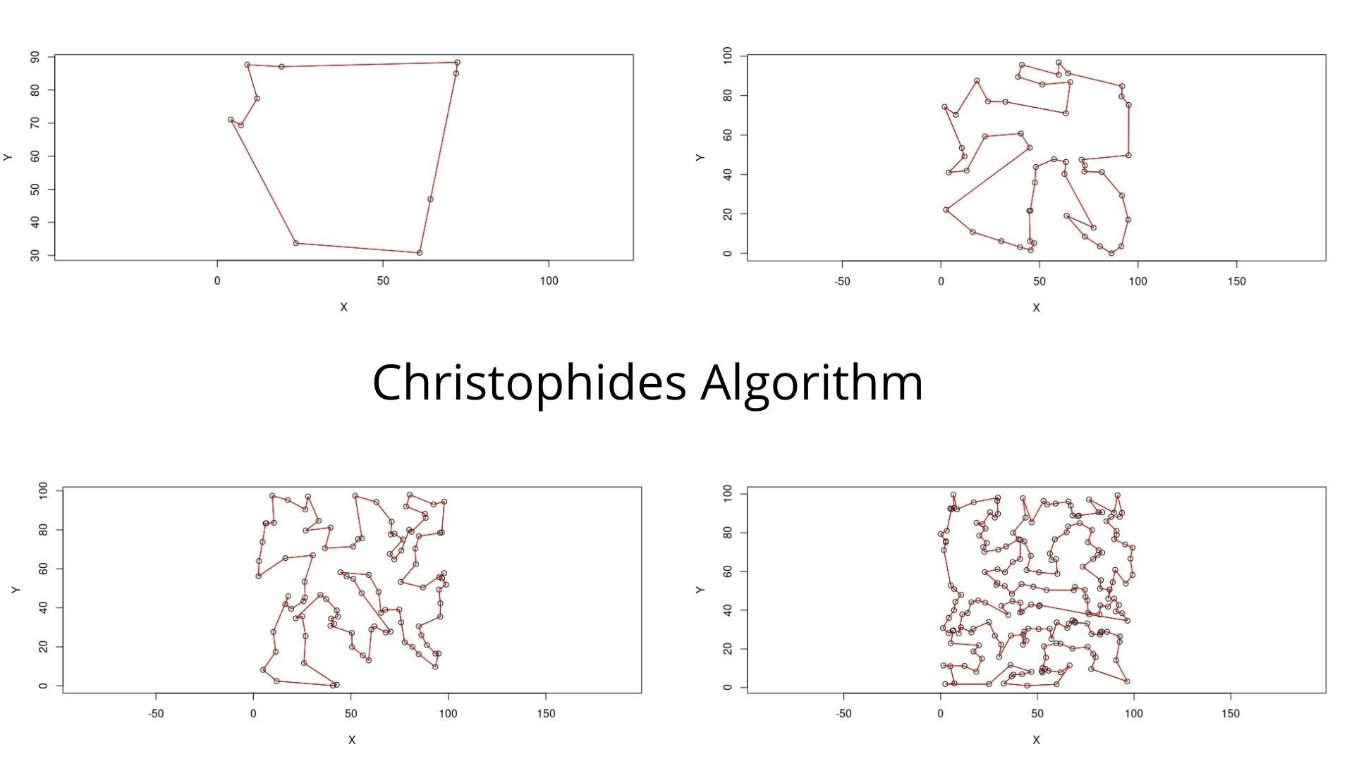Christofides Algorithm is an approximation algorithm that guarantees that its solution will be within a factor of 3/2 of the optimal solution length. Hence, it is also known as the 3/2 approximation / 1.5 approximation algorithm. It was discovered in 1976 by Nicos Christofides and Anatoliy I. Serdyukov. Firstly, we create a minimum spanning tree graph by using one of the many algorithms, such as Prim’s algorithm, Kruskal’s algorithm, etc. Then, we find all the odd-degree vertices(vertices with odd number of edges connected to them) and match these vertices, by the application of minimum weight perfect matching techniques. Then we combine these two graphs to form an Eulerian cycle (A cycle that visits every given node exactly once). To this day, this algorithm has provided the best approximation ratio that has been proven for the traveling salesman problem on general metric spaces.

Steps to code this algorithm:

• The input coordinates of the nodes can be provided in the form of a file or rather a random coordinate-generating function employing a certain distribution technique (normalized / uniform random distribution).
• Read the coordinates of the cities and plot them on a 2D graph.
• Calculate the Distance Matrix - an upper-diagonal 2D matrix that contains the euclidean distance calculated between all the cities taken in pairs.
• Construct the Minimum Spanning Tree (MST) - which is essentially a graph with no cycles and minimum possible weight (here euclidean distance). To implement Kruskal’s algorithm: We consider each vertex to be a separate tree. We traverse all the node pairs in the graph in the ascending order of distance. If two vertices are from different trees, we join these nodes and combine them into a single tree. On repeating this process for all the nodes, we obtain the MST of the undirected graph of nodes.
• Find all the odd-degree vertices in the MST.
• Match all the odd-degree vertices using minimum weight perfect matching techniques. There cannot be an odd number of odd-degree vertices, since each vertex must have 2 edges. Therefore, no vertices will be left out in this process.
• Construct a circuit by combining the MST and the perfect-matched edges. The resultant graph will have vertices with more than two edges (i.e. a single city might be visited more than once). We remedy this by removing repeating vertices.
• As an additional optimization step, we remove all the intersections by performing a simple Subtour reversal of nodes. We traverse all the edges of the graph and check for intersections with other edges. If an intersection is found between node x and y, we reverse all the list of nodes between x and y. We repeat this process until all the nodes are visited without correction.
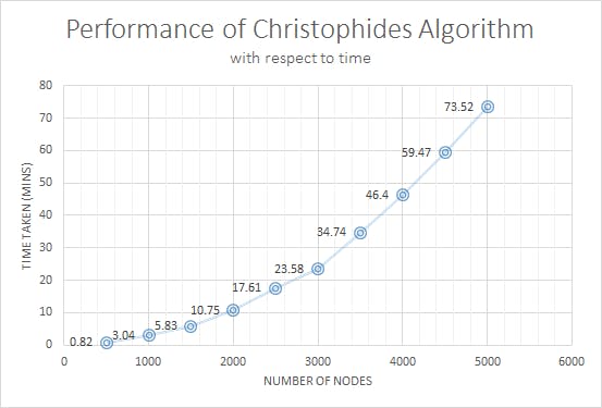
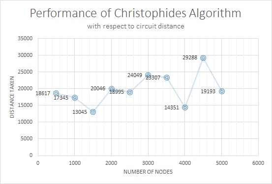
• Finally, we calculate the total distance covered by the tour and the time taken.
• Plot the solution path and save it in the output file.

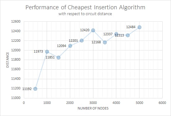
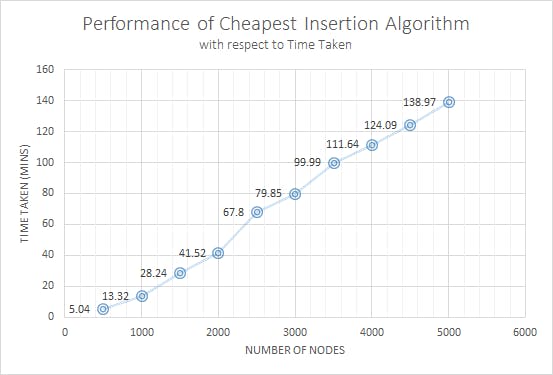
Cheapest Insertion Heuristic

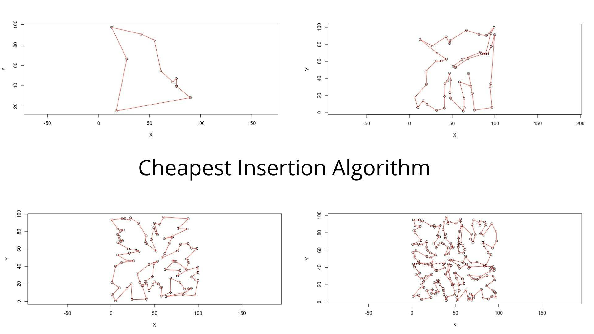
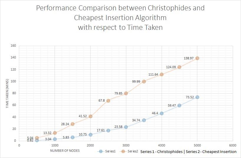
Cheapest Insertion Heuristic is an intuitive approach to the Travelling Salesman Problem. We start with a tour of small subsets of nodes and then extend this tour by inserting the remaining nodes one after the other until all nodes have been inserted. In case of The Cheapest Insertion Heuristics, among all nodes inserted so far, we choose a node whose insertion causes the lowest increase in the tour length. This algorithm provides mostly suboptimal solutions. But this solution can serve as a valid upper bound to further optimizations One of the biggest advantage of this method is that we do not tend to have the issue of crossover in between nodes and this provides a comparably optimal solution, whereas on the other hand, due to the number of iterations, this algorithm takes reasonably more time to provide the solution for the problem.

Steps to code this algorithm:

• The input coordinates of the nodes can be provided in the form of a file or rather a random coordinate-generating function employing a certain distribution technique (normalized / uniform random distribution).
• Read the coordinates of cities and plot them on a 2D graph.
• Calculate the Distance Matrix - an upper-diagonal 2D matrix that contains the euclidean distance calculated between all the cities taken in pairs.
• Construct a Convex Hull - the smallest convex polygon, that encloses all the given points (here cities), with the fewest number of points as its vertices. Mark the cities in the convex hull as visited.
• From the remaining cities, using the distance matrix, poll the city which is the closest to the convex hull. This ensures that the increase in weight (here euclidean distance) is small when added to the current set of cities.
• Now, we find the index of the tour path, at which the selected city must be inserted, so that we obtain the cheapest insertion cost. Insert this city into the set of visited cities and mark it as visited.
• Repeat Steps 5 & 6 until all the given input cities are visited.
• Calculate the total distance covered by the tour and the time taken.
• Plot the solution path and save it in the output file.

Comparison between both these algorithms:

A few input and output test cases are also committed in this repository under the test cases' folder, along with the circuit images. Feel free to clone the repository and play around with the code.

* These do not solve the problem, but provide valid upper bounds and approximation. But the word "solve" does look good doesn't it. 😀️
* All the distances are calculated with Euclidean path
** Time taken may vary with the speed of your processor.

Hope you learned something here. If yes, leave a 👍. நன்றி.